Cars are everywhere in games. They're a staple element of many genres, even in games that aren't strictly about cars. If a game world involves any sort of traversal, chances are there's a vehicle in it (unless you're deep in the realm of fantasy where you are riding a horse. The following will not cover programming horses, I apologize).
The special case of cars
The range of experiences that games offer through vehicles is massive. And that's what makes them fascinating to work with. Ever since I was a kid, I've played a variety of racing and vehicle games. I'd always chase the next racing title as soon as it hit the platform I had. But what struck me over time wasn't just the excitement of new cars or tracks; it was how different each experience felt, even though they all had cars at their core.
And here's the key insight: games are not physics engines. They are experiences. And racing games, more than many others, deliberately manipulate reality to deliver those experiences. With shooting games, for example, we expect certain behavior; bullets flying in straight lines, recoil, reloads. If those expectations aren't met, the game feels “off.” But with vehicles? There's an incredible amount of wiggle room.
Take Mario Kart. It's about as far from realistic driving as you can get; you're drifting on sand, tossing shells at your friends, and racing in a mushroom-powered go-kart that's all squashed proportions and cartoon physics. And yet it's beloved. It sells the fantasy of driving.
On the opposite end, you have full-blown simulators like iRacing or Assetto Corsa. Here, the experience is carefully crafted to reflect the nuance and challenge of real-life motorsport. People sink thousands of dollars into rigs just to replicate the feeling of being behind the wheel. And yet; both these games are programming cars at their core. They just prioritize different aspects of that experience.
So why the variability? Why can games get away with such a broad spectrum of driving models?
It's because when it comes to cars, we derive our expectations of them not just from first hand experience. Our understanding of what “driving fast” feels like is often built from second-hand sources; films, games, pop culture. We've all seen the hero of a movie shift gears a dozen times in a straight-line drag race. It's absurd, has nothing to do with reality, but it communicates something. It sells the feeling of acceleration, intensity, control. So kids get it; they want to “shift up” because it feels like doing something meaningful. It's the visceral feeling of controling something large and heavy at break-neck speeds.
So the key question for anyone implementing vehicles in a game isn't “what are the real physics I need to simulate?”, it's “what experience do I want to convey?”. From there you get to the question of “how do I implement that?”.
I've come to realize that the challenge of simulating vehicles in games lies in bridging two complex worlds: the experience and the machine. You need to understand both. Only then can you decide how and where to bend the rules; because game design isn't about simulating reality, it's about shaping it to fit your vision.
Chasing the Feel: The Iterative Path to AV-Racer
My first attempt at simulating a vehicle in a game was AV Racer, and it began as a simple top-down sprite using a basic Newtonian model. I controlled the car's movement with acceleration and braking, tied angular velocity to speed (so it wouldn't rotate on the spot), and called it a day.
Did it look like a car? Sort of. Did it feel like one? Not at all. It was more like a robotic puck skating around on invisible rails. So, iterating on that, I started hacking in some nonlinear curves and smoothing functions to mimic a behavior of a sliding car, trying to push away from the rigid feel. I faked the trail, exaggerated the drift, tweaked the angular momentum. It was all hacks, but it worked, somewhat. At least until Casey Muratori tried it and pointed out it looked like a car on ice, a spaceship. And he was right. It floated rather than gripped.
So I went back to the drawing board, already sunk in the hacky method, I added more magical numbers, created a parameter for “slidiness,” and kept tuning the system until it felt snappy, responsive, and fun. That final version is what I shipped on Steam. and you can read the technical breakdown of it in the devlog on my website here.
But here's the point: that car never really was a car. It was a clever trick, a cheat, an attempt to evoke the feeling of driving without simulating anything resembling the real thing. And that was okay, to a point, and it broke on edge cases. And if you give it to a racing driver or a sim driver they would immediately list all the things that are wrong with it.
What I learned from AV Racer is this:
If your goal is to capture the experience, you can get a long way without the real physics, but you'll always hit a wall.
There will always be an edge case, an awkward moment, where your system breaks the illusion. But more importantly, you're left limited by your own lack of understanding.
You can't convincingly bend reality until you know what you're bending it into.
Back to the drawing board
So after AV Racer, I decided to take a different path. I wanted to try doing it “right”; or at least understand what “right” even looked like. That meant diving deeper. I started researching actual vehicle dynamics, reading up on how cars behave in motion, and just as importantly, how drivers experience that behavior.
That shift; from faking to understanding changed everything. It became the basis for my next project, and it's what this talk (and this article) is really about: the intersection between how things work and how things feel, and what things you should care about to get a car in your game.
Throughout my journey trying to write this next engine, I was constantly stumped trying to tune out the noise between physics books and large repositories; what are the simplest high level concepts I need to understand and implement to get a simple vehicle on solid physical foundation? The goal of this talk, and article, is to help you, a developer interested in programming a car in their game, figure out where to start. And to give you the basic principles and list of things to care about while doing so.
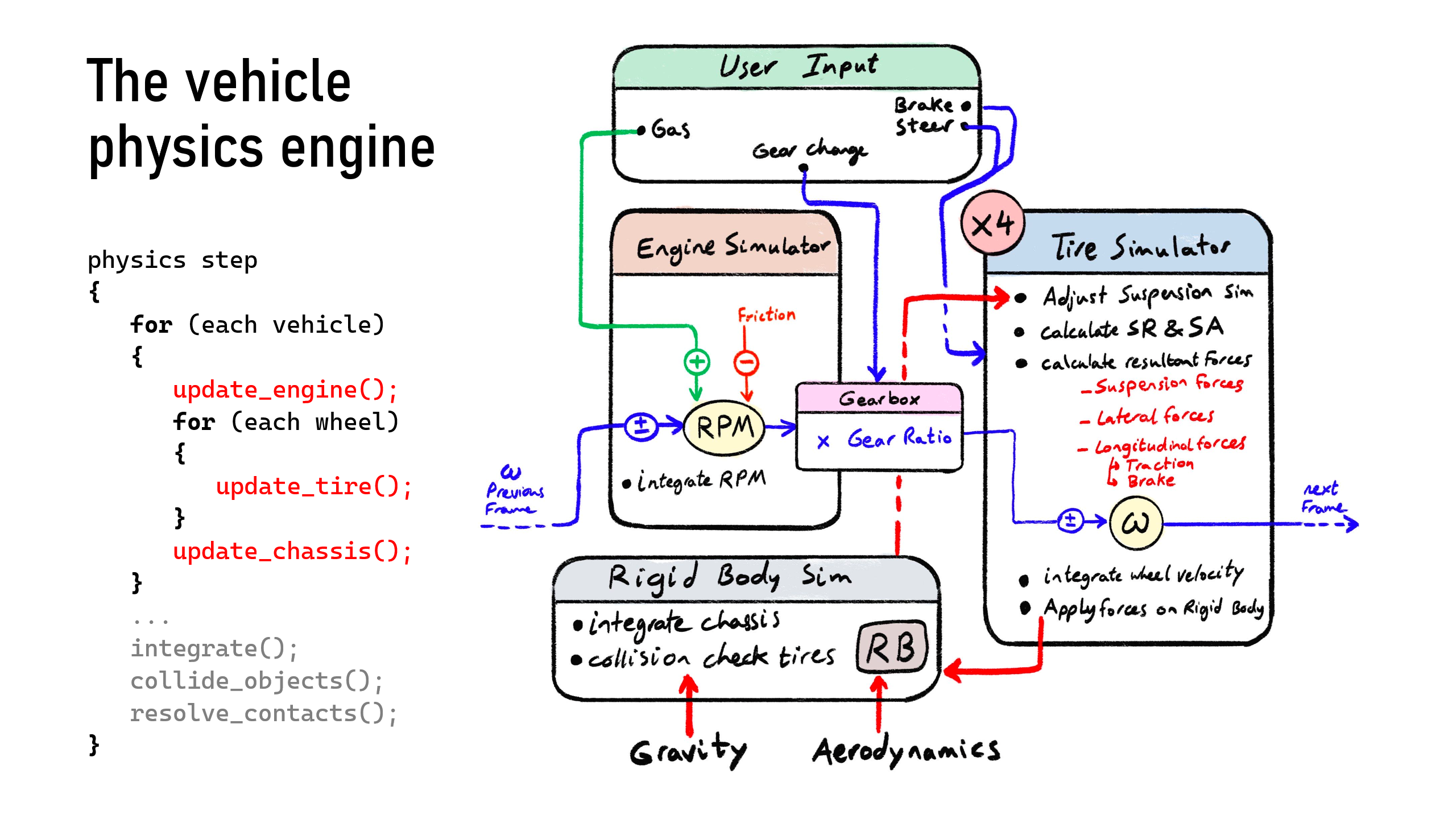
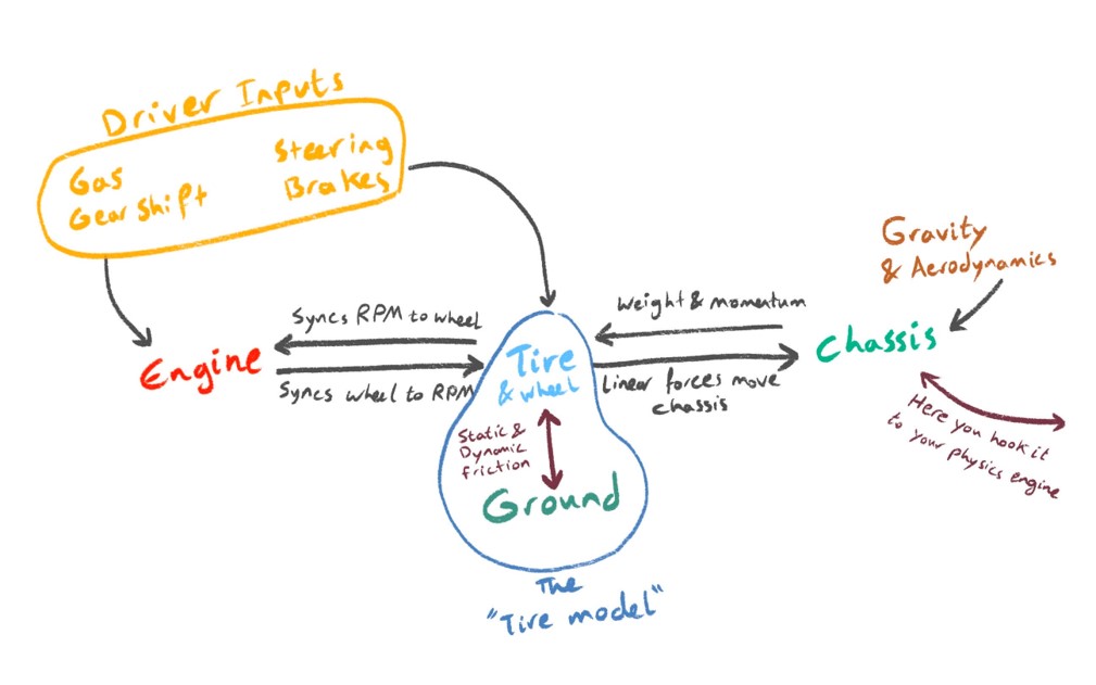
A Conceptual Model of Vehicle Simulation
At the core of it, a car in a game (at least one that behaves like a car) can be broken down into three main conceptual components:
1. The Engine (and Gearbox)
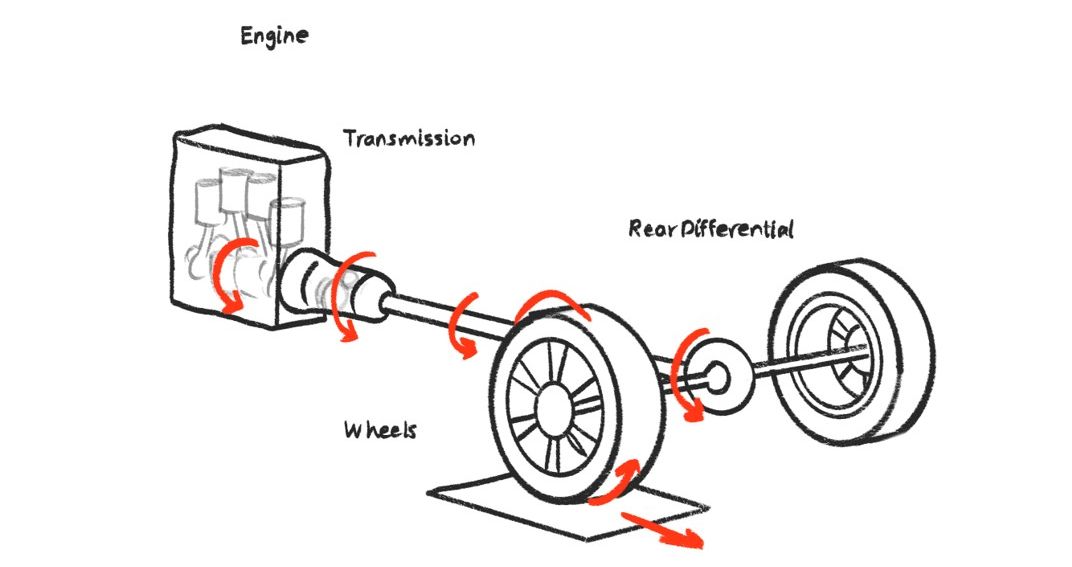
This is the logical starting point. When most people think of what “moves” a car, they think of the engine.
In our context, the engine also includes the gearbox, and together they form the unit that responds to player inputs like throttle and gear changes. At its simplest, the engine takes in throttle input and produces rotational speed and torque. That torque is then modified by the current gear ratio and passed on to the driven wheels. At the same time, the engine itself is also subject to feedback from the wheel speed, it doesn't spin in isolation. So there's a two-way sync happening here.
2. The Wheels and Tires
This is where the physics gets juicy.
The wheels receive torque from the engine. They also take in other inputs: brake input from the player, steering input, weight transfer from the chassis, and of course, friction with the road. This combination determines how much longitudinal (forward) and lateral (side) force the tires can generate.
But this as well is not a one-way system. The tires also affect the engine, because the actual wheel speed determines the engine speed. There's a feedback loop.
Now simulating the tire's interaction with the road is where tire models come into play. It's the tires that generate all the forces the car experiences. They are the only real contact point with the road, everything else is downstream from them.
3. The Chassis
The chassis is the simplest part to describe. It isn't a special problem to car physics to solve.
It's a rigid body that ties into the rest of your game's physics engine. It's the thing that actually moves. It responds to the forces from the tires, as well as external influences like drag, downforce, gravity, and collisions. And in turn, the chassis affects the tires by shifting the weight load across them as it moves and rotates. That, in turn, changes how much grip each tire has. Again, we're in feedback loop territory.
Component
Inputs
Outputs
The Engine (incl. gearbox)
Gas and shifter
Wheel speed
Sync. wheels to engine
The tire(s) (incl. wheels)
Engine speed & torque
Brakes
Steering
Weight load
Friction with road
Forces on the chassis
Sync. engine to wheels
The chassis (incl. body)
Forces from wheels
Aerodynamics
Weight on wheels
Everything moves with it
This all sounds complex, and it is. But the truth is, no game simulates all of this at full fidelity. Not even the most advanced racing simulators. Why? Because it's just not practical. You'd need full CFD (computational fluid dynamics) for air and fuel intake, real-time thermodynamics of tire rubber compounds, suspension dynamics, etc. No one's doing that except maybe a handful of automotive engineers locked in a lab at Porsche in Stuttgart.
So in game development, even with a physics driven model, we cut corners.
Some parts of the system are treated as black boxes: formulas that spit out plausible outputs based on reasonable inputs. Even in high-end racing sims, there's abstraction going on under the hood. There has to be.
So, ultimately there's no single “correct” way to implement vehicle physics. There is no Bible. No open-source silver bullet. Every game, every engine, every developer ends up carving their own path. So as a developer, you'll need to make choices, deliberate ones, about what to simulate, what to fake, and where to cheat. You won't get to say “I got the simulation right,” because there is no one right simulation. You'll have to design the system around what matters for your game.
Here is the general algorithm of how you would go through this in a physics loop in pesudocode:
So let's zoom into the first and perhaps most conceptually overloaded part:
The Engine
Interestingly, while the engine has the most moving parts in real life, in code, it's the simplest piece of the entire car simulation. Because at its core, the engine is just a torque calculator. It's concerned with producing a single output: rotational torque, from a set of inputs. It is essentially a blackbox.
But to get this right, and to make it feel right, we have to understand the mechanics behind the numbers.
Let's look at a simple example:
Stage
RPM
Torque (Nm)
Power (kW)
Force (N)
Engine
5000
200
100
n.a.
Transmission (1:3.5)
1428
700
100
n.a.
Differential (1:4.1)
380
2870
100
n.a.
Wheels (r = 0.3m)
380
2870
100
9566
suppose we have an engine producing a flat 100 kW of power at 5000 RPM. That translates to about 200 Nm of torque. But that speed is way too fast for the wheels to handle directly. So, enter the gearbox and differential, which scale down the speed while boosting the torque. By the time the force reaches the wheels, after a gear ratio of 4.2 and a differential ratio of 3.8, you would end up with something like 9500 N of linear force (after converting torque through wheel radius). That's a lot of grunt at the contact patch. Understanding this is essential because torque is not fixed. It changes based on the engine's RPM, and how that engine is connected to the drivetrain.
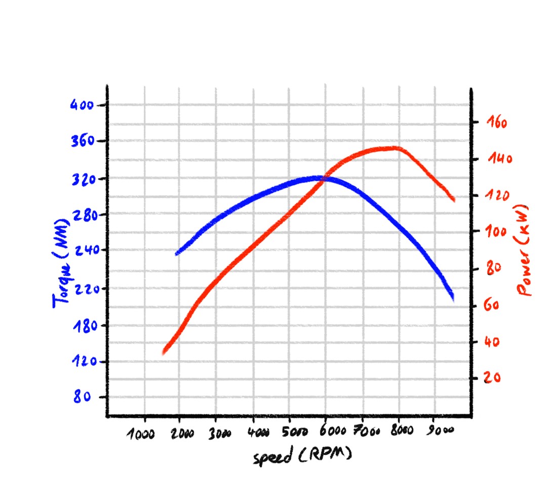
Now if you're into tuning cars you will recognize this iconic image:
A torque curve rising and falling next to a similarly shaped power curve. These two hills represent the output characteristics of an engine across its RPM range. Torque tells you how strong the engine is at any moment. Power is the result of torque times RPM (with some constants in between). Each engine has its own "personality": some peak early and drop off, others ramp up slowly and scream at high revs. These shapes affect how a car feels to drive. A snappy, torquey low-RPM engine feels wildly different from a peaky high-RPM screamer, even if both cars hit the same top speed.
Key take is this: The engine's power output is variable at different speeds.
Ok, good, now how do you simulate that? How do I put it into code?
You don't need to simulate combustion cycles or real torque output. What you need is a curve that gives believable values based on RPM. So here's what I did: I opened up Desmos, sat there for an hour, and built an abomination:
\[ y = (a - b) \cdot e^{\frac{-(c(x - d))^2}{f^2}} + b \]
a: adjusts curve baseline y b: adjusts peak magnitude
c: adjusts ends slope
d: adjusts peak x position
f: adjusts ends slope
I reverse-engineered a torque curve formula; not from real data, but from visual tinkering. I created parameters I could play with.
This gave me knobs to control. The goal wasn't 1:1 simulation, but realistic experience and tunability. The result was a black-box function that gets plugged into the engine simulation and makes your virtual motor come alive with character. With a few tweaks, you can simulate anything from a diesel truck to a screaming F1 car:
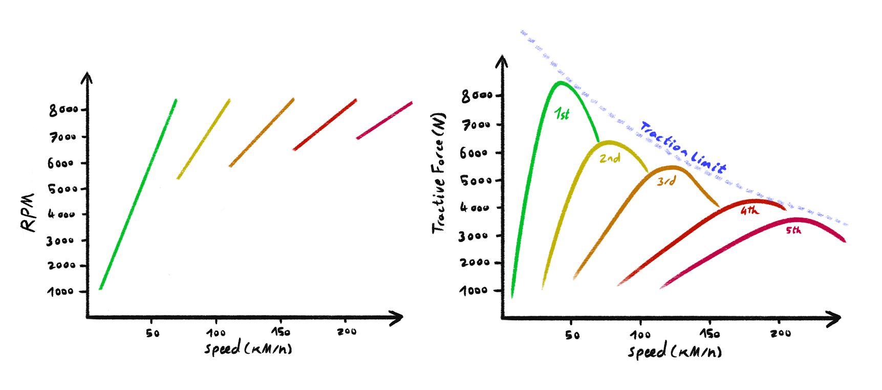
The Gearbox
The gearbox is dead simple: it's a lookup-table of ratios. Each gear multiplies the engine's output torque and divides the RPM. The player shifts gears, and you look up the current ratio. That's it. But the result of this mechanic is huge in terms of how a car accelerates. It defines your acceleration profile, top speed, and how much freedom you give the player to manage the engine's sweet spot.
The gearbox is dead simple: it's a lookup-table of ratios. Each gear multiplies the engine's output torque and divides the RPM. The player shifts gears, and you look up the current ratio. That's it. But the result of this mechanic is huge in terms of how a car accelerates. It defines your acceleration profile, top speed, and how much freedom you give the player to manage the engine's sweet spot.
Gear
Ratio
R
-2.92
N
0
1
2.50
2
1.61
3
1.10
4
0.81
5
0.68
Implementing the engine and drivetrain: From Curve to Code
There are two key state variables to manage, and they're codependant:
The engine RPM
The driven wheel's angular velocity
The engine and the wheels constantly push and pull each other toward equilibrium. It's a differential equation you'll need to solve in code.
Expected angular velocity for the current engine RPM in current gear.
\(\omega_t\)
Current angular velocity value.
One key aspect to solving the codependency between these two variables is observed in \( (R_{ex} - R_t) \) and \( (\omega_{ex} - \omega_t) \) respectively. It is a neat solution suggested to me by Demetri Spanos to deal with the differential equation. It basically turns the coupling into two “chase the target” terms. \( (R_{ex} - R_t) \) says “how far is the engine RPM from what the wheels demand right now?”, and \( (\omega_{ex} - \omega_t) \) says “how far are the wheels from what the engine is trying to spin them at?”. Each difference becomes a proportional drive term in its respective differential equation, so you can step them sequentially each frame without solving a fully coupled system. Because each step uses the most recently updated value of the other variable, the system converges toward consistency frame by frame. If you need tighter coupling, you can iterate the two updates a couple of times per frame, and so on. Stability-wise, just keep dt small relative to your gains (k) so you don't overshoot.
What makes this elegant is that you can scale complexity as needed. Keep it simple for arcade games, or layer on more realism if you're going for a sim. The foundation remains the same, engine rpm and wheel angular velocity are connected.
It is important to note, that this is the solution I have reached by the time I wrote this article. You might find a better way to do this, and if you do, I would be happy to learn about it, just shoot me an email!
Putting it together, here is a demonstration from my engine (you need sound for this):
Once the torque curve system is in place, you can take advantage of its easy tweakability with cheap to introduce depth.
In this demonstration from my current engine you could see familiar terms from the world of car engines: bore, displacement, camshaft profile, turbocharger. These don't exist in the physics model at all. Each of these terms was mapped to one of the parameters in my torque curve function. Changing the "cam profile" might shift the peak of the curve. Adjusting the "displacement" might increase baseline torque. These were essentially just control knobs with labels that made sense for the player. So while it's not a true simulation of engine mechanics, it creates a meaningful interaction: if you adjust a parameter, you see and hear a change in behavior. It gives the impression that you're tuning a real engine. The goal here isn't necessarily accuracy but rather to establish a clear cause and effect between what the player modifies in gameplay and what the car does.
I also tied these parameters into the sound system, so changes to the engine affected not just performance, but also how the car sounds. That way, when someone upgrades the turbo in the shop, they get more than just numbers, they hear the result as well.
The Tire Model
With the engine covered, we move to what I consider the most critical component of a racing simulation: the tire.
It's where all inputs are translated into action. And in a racing game, if the tires aren't programmed right, nothing will feel right.
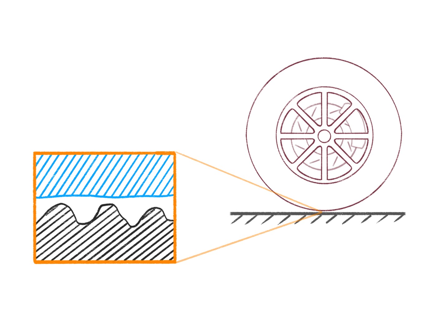
Getting tires right is essential because they are the only part of the car that actually touches the road. All forces: acceleration, braking, turning, are transmitted through that small contact patch. It's the source of all feedback, control, and physical realism.
Modern tires are a complex piece of engineering. We've come a long way from the invention of the wheel, particularly since the discovery and use of vulcanized rubber, which introduced controlled elasticity into the system. That elasticity is central to how tires generate force.
Here's the basic principle:
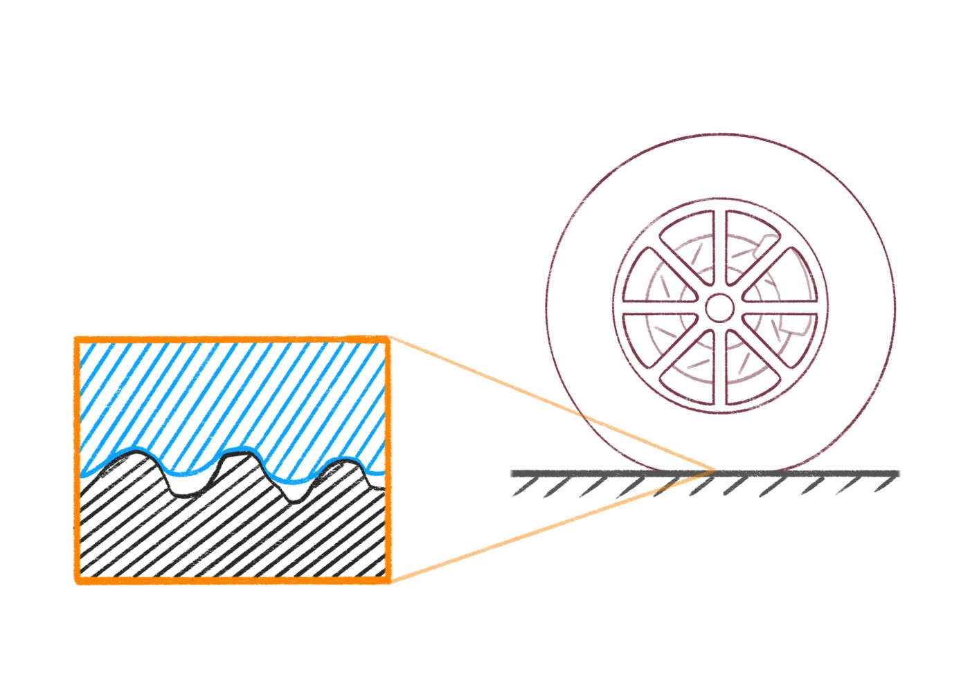
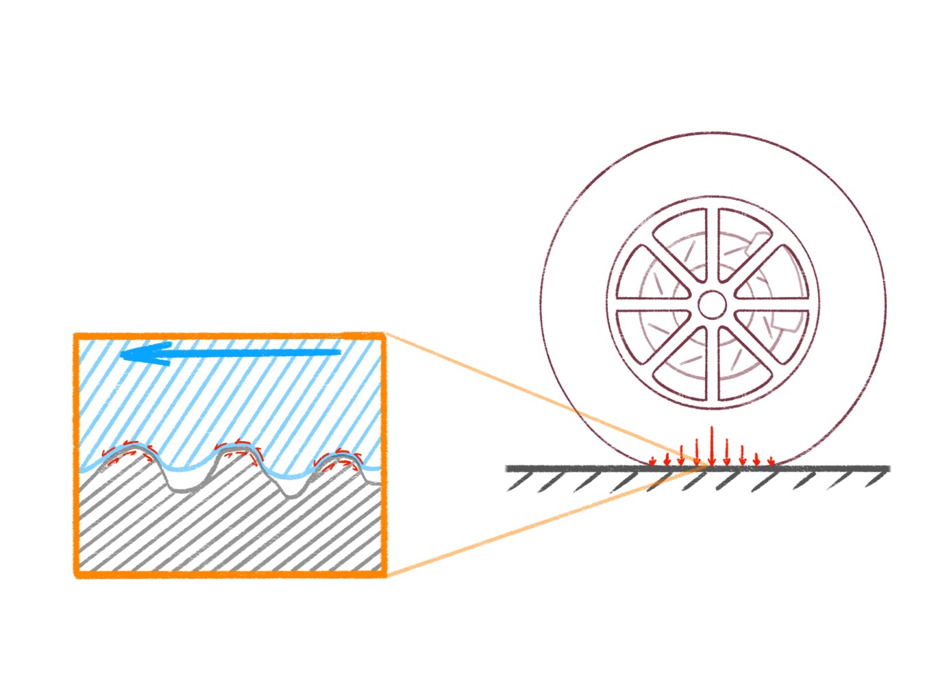
As the rubber contacts the asphalt, it deforms slightly under load. That deformation creates elastic forces within the tire. As the car moves or the tire rotates, that elasticity resists shear, which in turn creates the traction force that accelerates or turns the vehicle. To visualize this at a micro level, think of the tire tread “gearing” into the texture of the road; into the tiny peaks and valleys of the asphalt. When the tire is pressed down by the car's weight (normal force), it begins to grip the road surface through this deformation. As long as this interaction remains within the limits of the rubber's elasticity, the tire is in static friction, which is what gives the car control and grip.
But elasticity isn't infinite. Push the tire too far, by turning too sharply, accelerating too hard, or locking up the brakes, and the contact patch deforms past its elastic limit. At that point, the tire transitions to dynamic (or kinetic) friction, and starts sliding across the road. That's when grip is lost, and control becomes difficult.
Understanding this transition is key for simulating the tire's behavior during acceleration, braking, and turning. It's also what makes tire modeling one of the hardest parts to get right.
Imperically there is a maximum force a tire can physically generate on a car under certain conditions, beyond that, and the tire's elasticity limits are reached and it starts sliding on the road. To understand this, we can break sum of the forces generated by tire friction with the road into longitudinal and lateral components. We can express this relationship as:
\[
F = \sqrt{F_x^2 + F_y^2}
\]
Longitudinal Tire forces
The first concept to understand here is static friction.
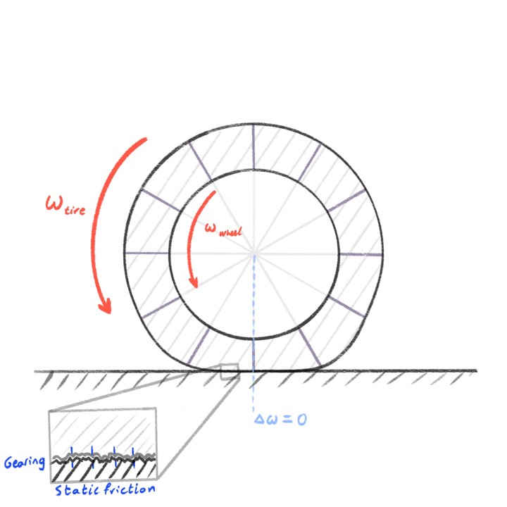
Let's start with a basic example: a tire rolling down the road at a constant speed, with no throttle or braking. In this case, the angular velocity of the wheel hub matches the tangential velocity of the contact patch on the road. There's no sliding; just rolling. The tire deforms slightly through the weight it's carrying, and grips the road through static friction, and everything is in balance.
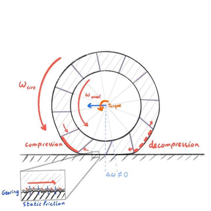
But what happens when you press the throttle? When you apply power, the driven wheel starts rotating faster than the tire would on its own. That difference creates a twist in the rubber.
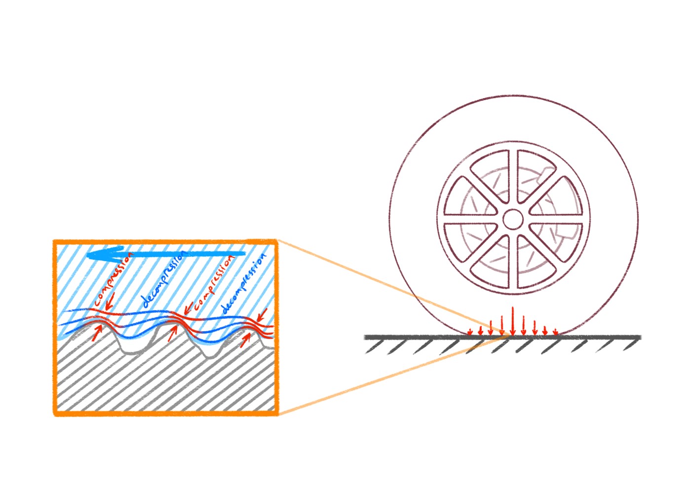
The contact patch deforms: compression zones form toward the front, decompression zones at the rear. This deformation stores elastic energy and produces a force that pushes the car forward.
As long as this remains within the tire's elastic limits, you're still in the realm of static friction.
But push further (apply more power, or reduce grip) and eventually that deformation exceeds what the rubber can handle.
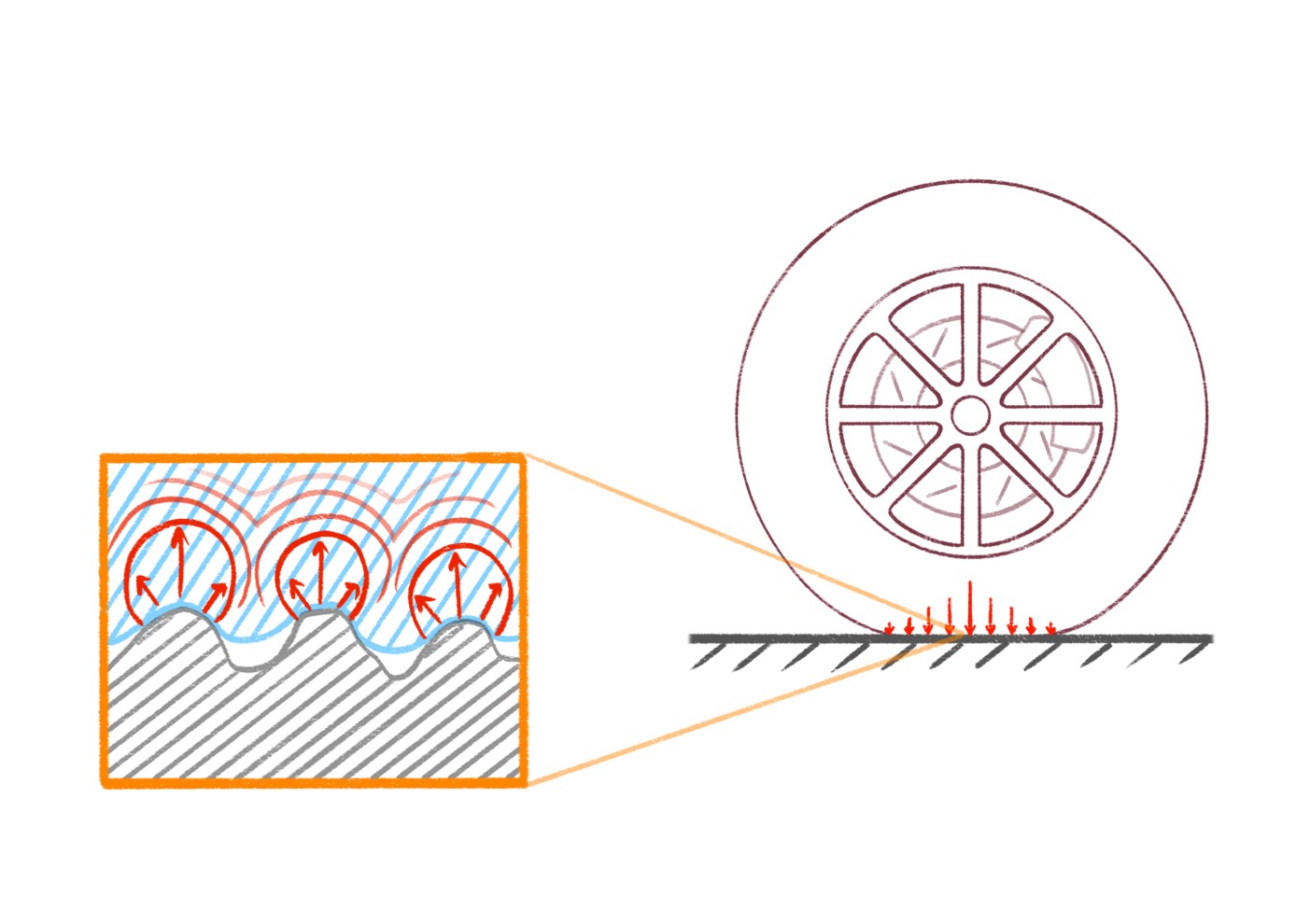
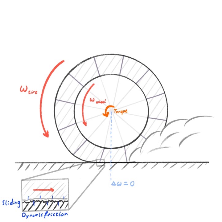
At this point, the tire starts to slide, entering the domain of dynamic friction.
This transition is crucial: it's where traction starts to fall off and control begins to degrade.
Static friction: the tire is gripping the road. There's deformation, but no sliding.
Dynamic friction: the grip has broken. The tire is now sliding across the road surface. Once that threshold is crossed, the available friction drops sharply.
The Slip Ratio
The transition between those two is where the interesting part happens. The difference between how fast the wheel wants to spin and how fast the car is actually moving along the ground is exactly what determines longitudinal tire force. That difference is captured in a value called the slip ratio.
Now, personally, I find the term a bit misleading. It implies a measure of how much the tire is "slipping", when in reality it's more of a measure of deformation in the longitudinal component. But it's the accepted terminology in tire dynamics, so we'll stick with it.
Slip ratio is a unitless value that quantifies the difference between the rotational speed of the wheel and the speed of the vehicle along the ground. If both are perfectly matched (no power applied, no braking) then the slip ratio is 0. As soon as the wheel starts rotating faster than the vehicle is moving (acceleration), or slower (braking), you get a non-zero slip ratio.
This is where the tire begins to deform and generate usable force.
from Society of Automotive Engineers document SAE J670 “Vehicle Dynamics Terminology”
Or alternatively as:
\[
SR = \frac{\omega R_l}{V} - 1
\]
\(\omega\)
Angular velocity of the driven/braked wheel
\(R_l\)
Loaded radius of the wheel
\(V\)
Linear velocity of the axle over the road surface
from Calspan Tire Research Facility
(there are many different ways to define it, they all map more or less to the same thing)
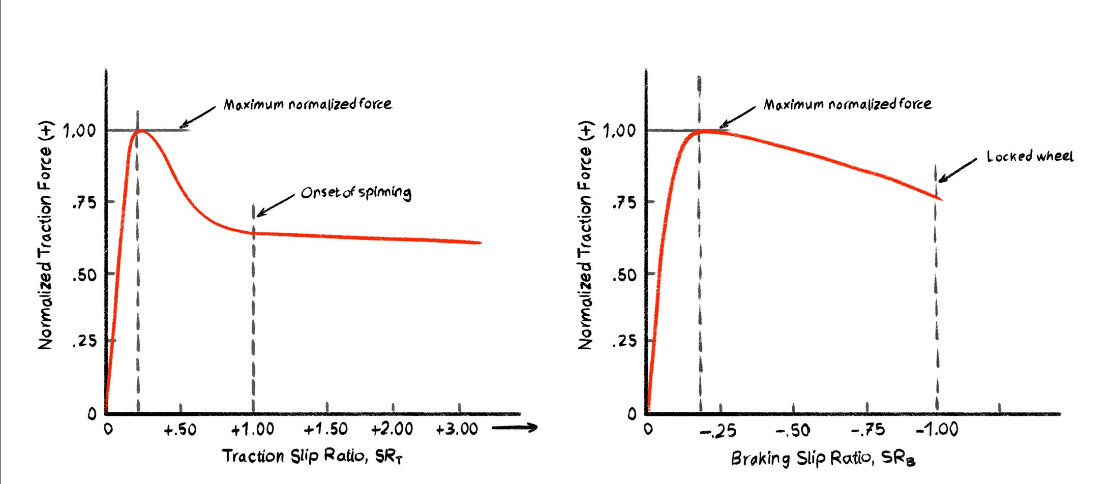
Now if we plot the the slip ratio against the longitudinal force generated by the tire. The result is a curve:
At low slip ratios, traction increases with more deformation; this is the tire flexing and gripping the road.
At a peak, the tire reaches its maximum traction.
Beyond the peak, the tire begins to slide, and force drops off; this is dynamic friction.
Even when fully slipping, the tire still generates some force (e.g., spinning out still moves the car forward slightly).
In braking, the behavior is similar. Locking the wheels completely doesn't eliminate all stopping power; it just makes it much less effective. The curve tends to drop more gradually in braking, due to how rubber compresses under deceleration.
It's important to clarify something: a non-zero slip ratio does not mean the tire is sliding.
You can have a moderate amount of slip and still be in static friction; that's the sweet spot where real driving happens. This entire process is a spectrum, not a binary state. Grip transitions fluidly from perfect rolling contact to full slip, and the physics engine should reflect that. Good simulation happens in this middle ground, where the tire is deforming but not yet sliding. That's where control, feedback, and vehicle responsiveness come from.
Once you understand the physical principles, the code is actually pretty manageable. You need:
A way to compute slip ratio (difference between tire rotation and vehicle speed)
A function to turn that slip into a force scaling factor
Now to convert the slip ratio to a curve we use a similar apporach to the fucntion I mentioned earlier for the torque curve. For this one use a formula created by Hans B. Pacejka (1934-2017). He was a Dutch vehicle dynamics engineer who became legendary in the world of tire modeling. A professor at Delft University of Technology, he authored tire and Vehicle Dynamics, which remains a staple reference in automotive engineering. He has devised a "Magic Formula" also known as the “Pacejka tire model,” this empirical relationship captures complex tire behavior using a compact sine/arctangent function with enough knobs to give full control over its behavior:
\[
y = D \cdot \sin\left( C \cdot \arctan\left( Bx - E \cdot (Bx - \arctan(Bx)) \right) \right)
\]
If you calculate and adjust this behavior for each wheel, the results can be quite interesting:
In this case, the rear wheels spin significantly faster than the vehicle's forward speed. The slip ratio is high, and the traction force is low; classic loss of grip.
In this case, there's mild, controlled slip as the player gently applies the throttle. The wheels and ground stay relatively synchronized, generating strong forward force. That's the ideal case when driving.
These are the kinds of emergent behaviors you get from modeling slip ratio correctly. Even a simplified model, when done right, can give you the feedback and realism that make a car feel right.
Lateral Tire forces
So far we've looked at how tires behave in the longitudinal direction; accelerating and braking. Now we focus on lateral forces, what happens when a car turns, Or more precisely, when a tire turns away from where it's headed.
When a wheel turns, the contact patch doesn't stay rigid. It deforms. That deformation, caused by lateral loads, is what generates the force that steers the car.
To simulate this behavior correctly, we need to understand a few angles:
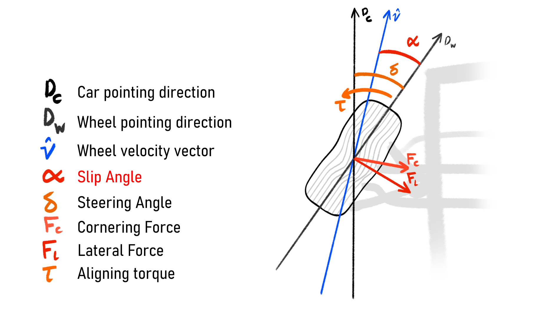
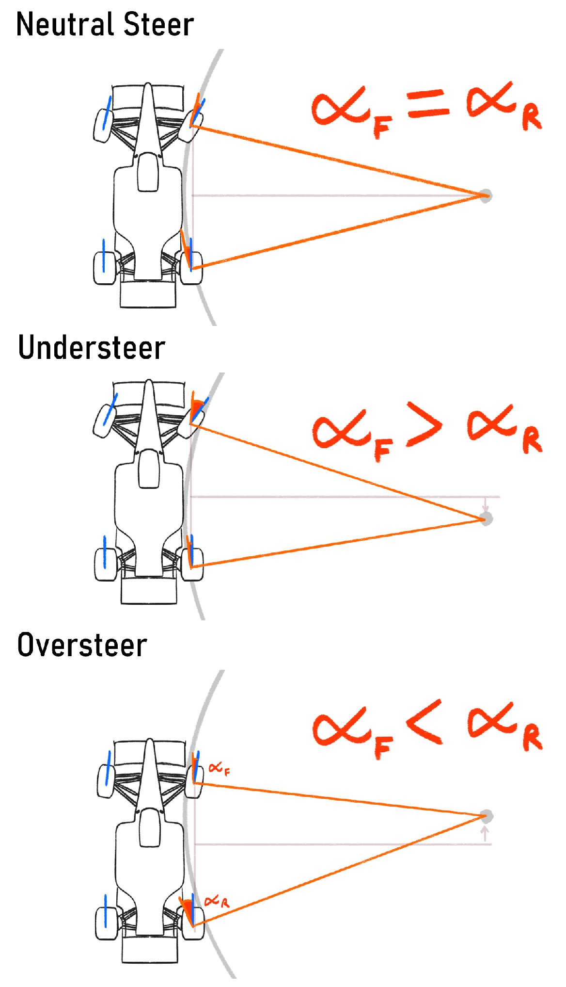
In this graph we're looking at the front-left tire of the car, from above. The car's body is pointing in one direction (Dc), the tire is physically steered in another (Dw), and the car's actual movement through space (its velocity vector V) might point somewhere else entirely; due to yaw, side forces, or rotation. From these vectors, we extract two important angles:
Steering angle: The difference between the car's forward direction and the direction the wheel is pointing. Slip angle: The angle between the wheel's pointing direction and the velocity vector of the tire.
Careful though: the Slip Angle is not to be confused with Slip Ratio, which refers to wheel spin in the longitudinal direction.
The Slip Angle governs lateral force, The Slip Ratio governs longitudinal force.
The terminology is very confusing, but unfortunately, it's standard.
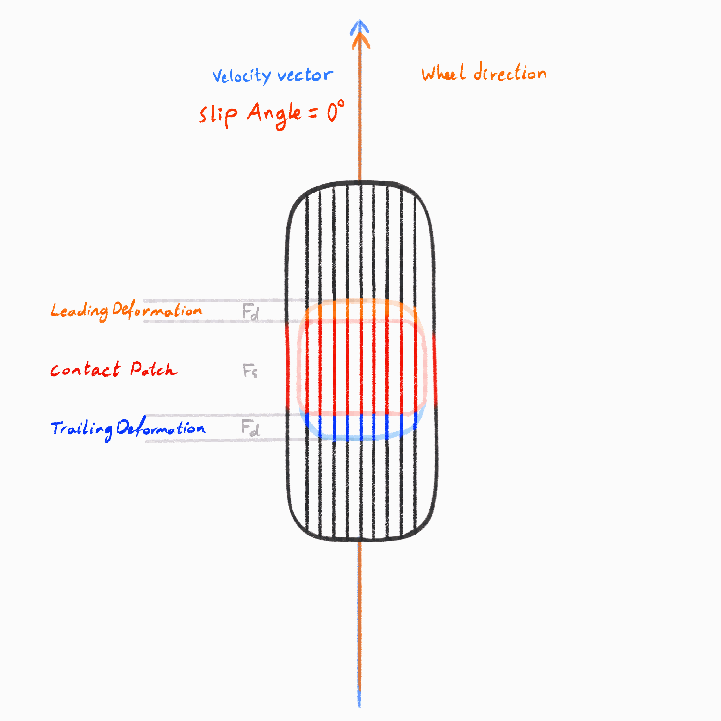
When a tire is loaded laterally (i.e. when the car is turning) the rubber again deforms. The leading edge of the contact patch leads to an area in full static friction, fully gripping the road. But as you move across the contact patch toward the trailing edge, you enter a gradient of deformation that eventually exceeds the rubber's elastic limits. At the trailing edge, dynamic friction dominates, and the tire begins to slide.
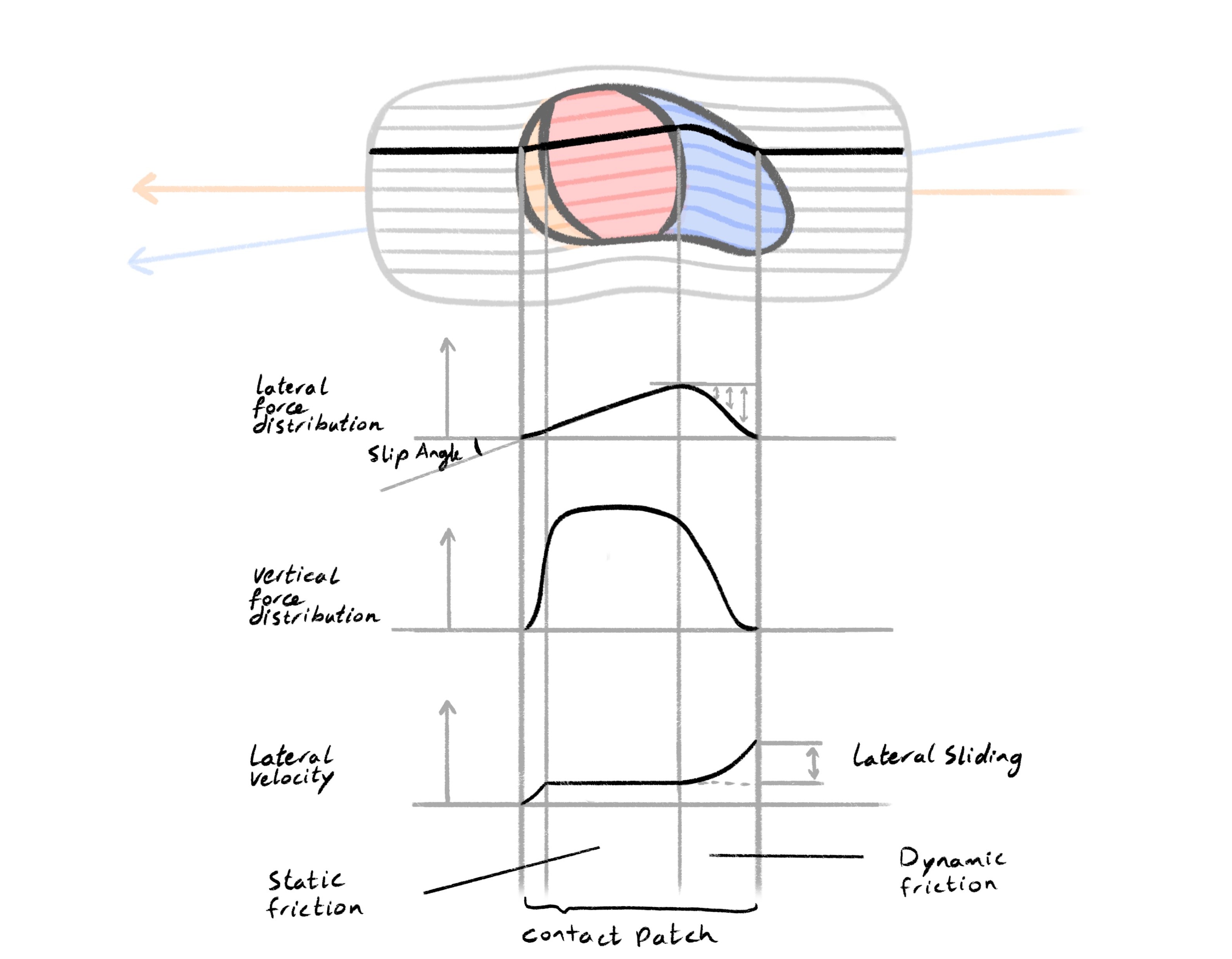
This diagram illustrates how lateral force builds and breaks down within a tire's contact patch during cornering. As the wheel is steered at a slip angle, the tread elements enter the patch slightly misaligned with the direction of travel. The black centerline of the tire's heading deviates from the path it's actually following — this difference is what generates lateral force.
At the of the contact patch, the tread converges from dynamic into static friction. In the middle The rubber sticks to the road and deforms laterally, twisting the tire carcass and building up lateral shear force. This force rises progressively, as reflected in the lateral force distribution curve.
Roughly two-thirds into the patch, the tread reaches its grip limit. Beyond this point, it can no longer maintain static contact and begins to slide, entering the dynamic friction again. As a result, the lateral force tapers off, and the tire starts to lose grip. Meanwhile, the lateral velocity graph at the bottom shows a sudden increase; the tread is now moving relative to the ground.
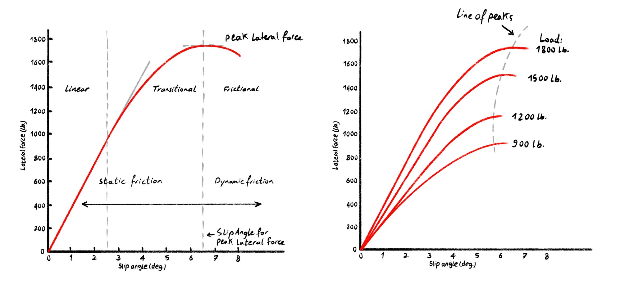
The vertical force distribution in the center graph reveals another layer: the tire isn't pressing down evenly. Load builds near the front of the patch and decreases toward the rear, meaning the available grip is also uneven. This interplay between deformation and sliding explains the well-known shape of the lateral force vs. slip angle curve, a gradual rise, a peak, and then a falloff, all rooted in the physics of the contact patch.
Advanced tire models simulate this in detail, dividing the contact patch into many discrete zones, each with its own response curve. For example this is what research groups like Calspan and commercial projects like BeamNG drive do. But for most gameplay goals, you don't need this level of granularity and can get away with one simulated point per tire patch.
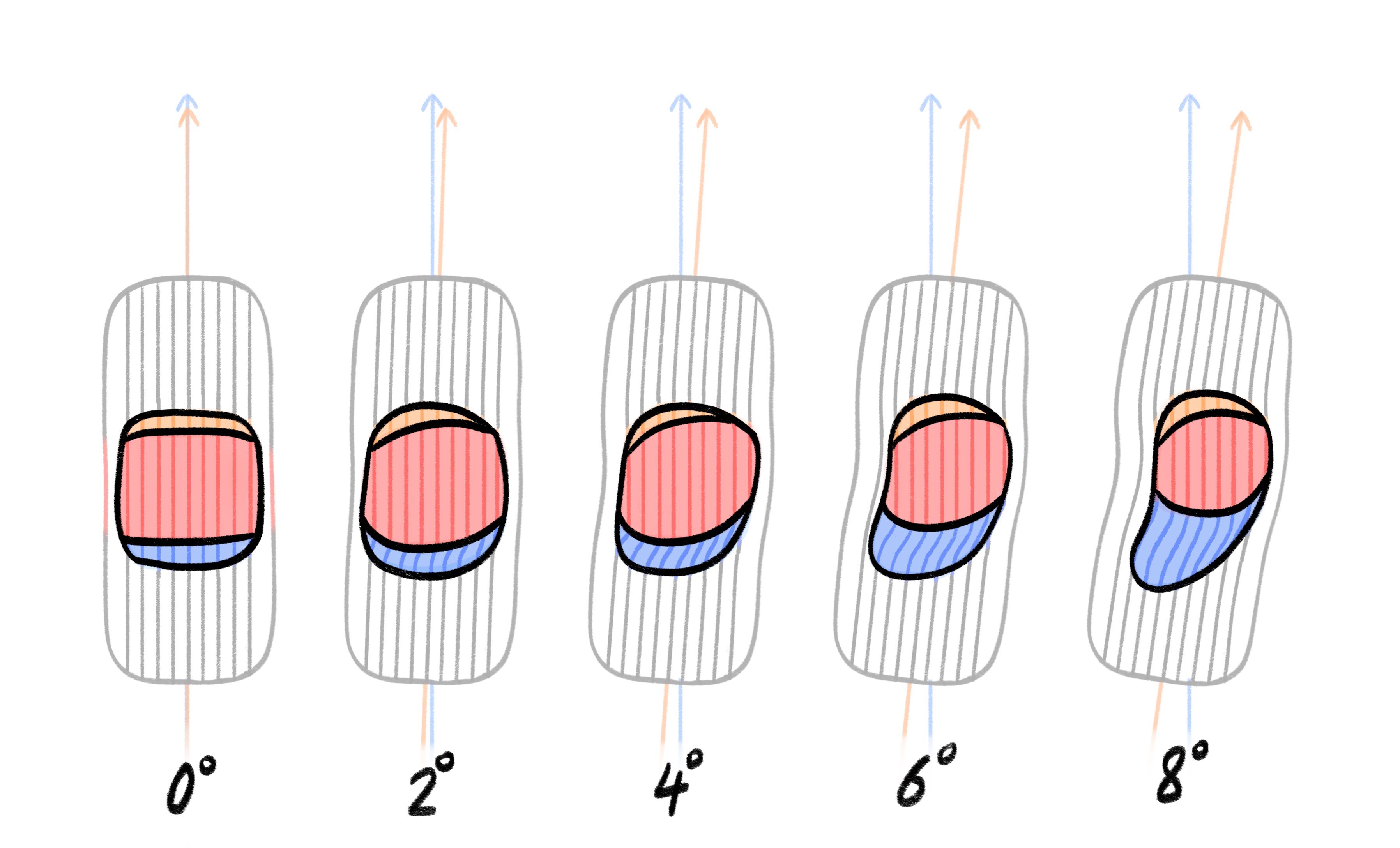
The center of the patch is where static friction dominates. The edges are where deformation begins and the transition from dynamic friction to static friction happens. As slip angle increases, the effective size of the contact patch shrinks until it's almost entirely sliding.
The real-world consequences of slip angle show up in familiar driving behavior:
Neutral steer: This is the balanced case where the slip angles are roughly equal at both the front and rear axles. As a result, the car turns precisely as the driver intends. This condition is often the design goal for race cars at mid-corner speeds.
Understeer: The front tires develop larger slip angles than the rear. This means they reach their grip limit sooner and begin to slide, causing the car to follow a wider arc than what the steering input suggests. The vehicle resists turning, and the driver must either reduce speed or increase steering input to stay on course.
Oversteer: voccurs when the rear tires generate more slip angle than the front, they lose grip earlier and start to slide outward, causing the rear end of the car to swing out. This can feel unstable or result in a drift, especially if not corrected with steering or throttle input.
What's important here is that you don't need to hard-code these behaviors into your simulation. If your tire model responds correctly to slip angle and load, these handling characteristics emerge naturally from the physics. In AV-Racer, I used hardcoded logic to fake understeer and oversteer transitions. But in this newer system, they arise organically as a result of tire forces, slip angles, and weight transfer, just like in the real world.
Just like with slip ratio, lateral force also follows a curve:
As slip angle increases, lateral force increases. A peak is reached. Beyond the peak, force falls off as more of the patch transitions to dynamic friction.
This curve's shape is influenced by the vertical load on the tire. More load generally increases total available grip; but not linearly. This phenomenon, known as load sensitivity, is why tires perform differently under cornering, braking, and weight transfer.
As with longitudinal forces, we can use a simplified function to approximate lateral behavior. Again, you can use Pacejka's Magic Formula for this. You calculate the slip angle, plug it into the formula, and get a scalar that defines how much lateral force to apply.
You can notice that a lot of those parameters are very dynamic, and the emerging realization that comes from working on this is the following:
The more parameters you let change dynamically, and the more those parameters are rooted in real-world mechanics, the more believable your simulation will feel.
Here is a demostration from my current game engine where I change the slip angle curve parameters on the fly which results in different emergent behavior to steering stability, from understeer to oversteer:
Combining the longitudinal and lateral components
Now we come to what is, in my experience, the most conceptually difficult part of vehicle simulation: understanding the relationship between longitudinal and lateral tire forces, and how they limit each other.
This is where many simplified models fall short, and where most realistic ones start to show their complexity. It's also where the tire starts to feel like a single, dynamic unit, not two separate force systems glued together.
Throughout this article, we've been treating longitudinal force (acceleration and braking) and lateral force (cornering) as separate systems, each with its own inputs; slip ratio and slip angle, respectively. But in reality, each tire produces one combined force vector that is a function of both slip components.
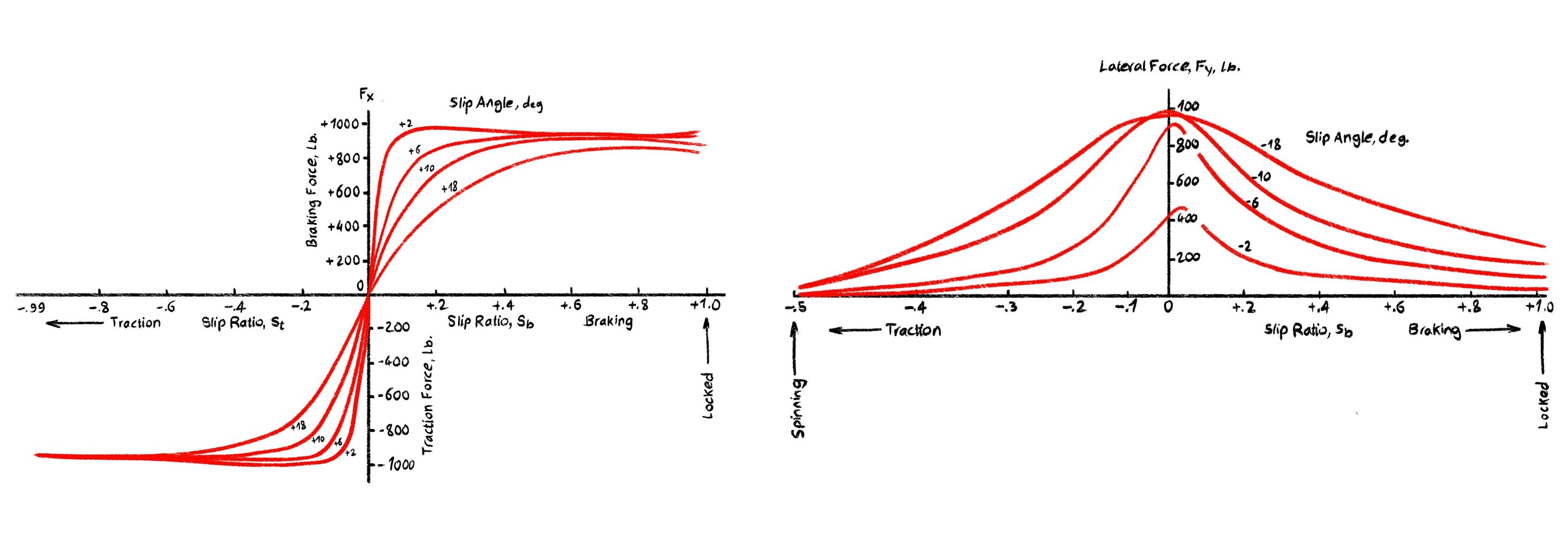
These two graphs show how a tire's ability to generate grip changes when it's asked to handle both braking/acceleration and cornering at the same time, i.e. "combined slip". One could observer that a tire has a limited force budget, and using it in one direction reduces what's available in another.
The left graph shows how longitudinal force (traction or braking) changes with slip ratio at various slip angles. At 0° (no cornering), the tire can apply maximum braking or traction. But as slip angle increases (i.e. the tire is turning), the available longitudinal force drops. At +18°, the tire is so busy cornering it has little grip left for acceleration or braking. This is why hard braking mid-turn can cause instability.
The right graph shows the opposite: how lateral force (cornering) varies with slip ratio. Peak lateral grip happens when the tire isn't under heavy braking or acceleration. As slip ratio increases, lateral force drops off — at extreme slip ratios (like locked brakes), the tire can barely corner at all.
This illustrates a fundamental truth of vehicle and racing dynamics: you can't brake and turn at full force simultaneously. A good tire model needs to account for this tradeoff.
Now plotting longitudinal forces and their corresponding slip ratio on one axis and lateral force and corresponding slip angles on the other and plotting the combined force we get this:
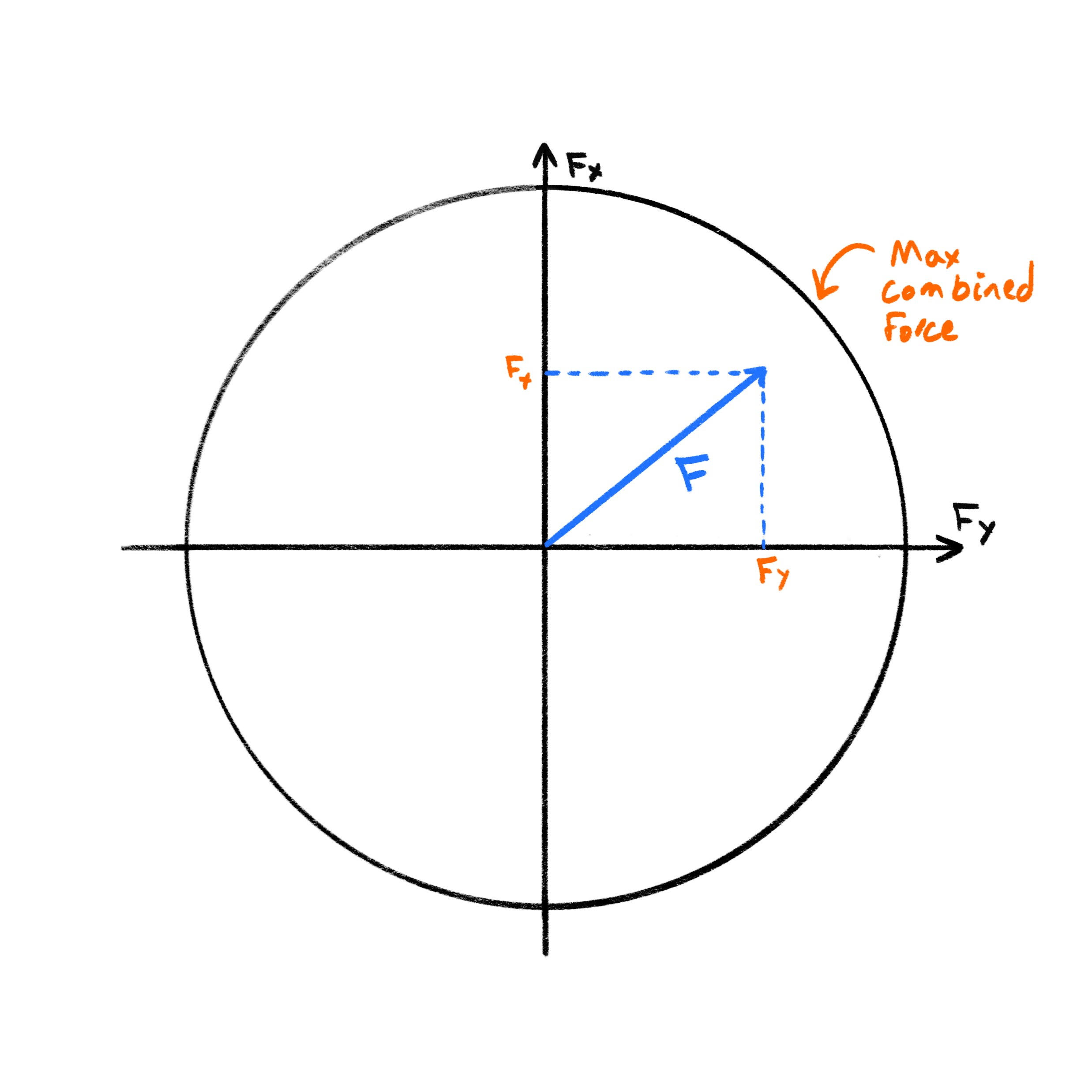
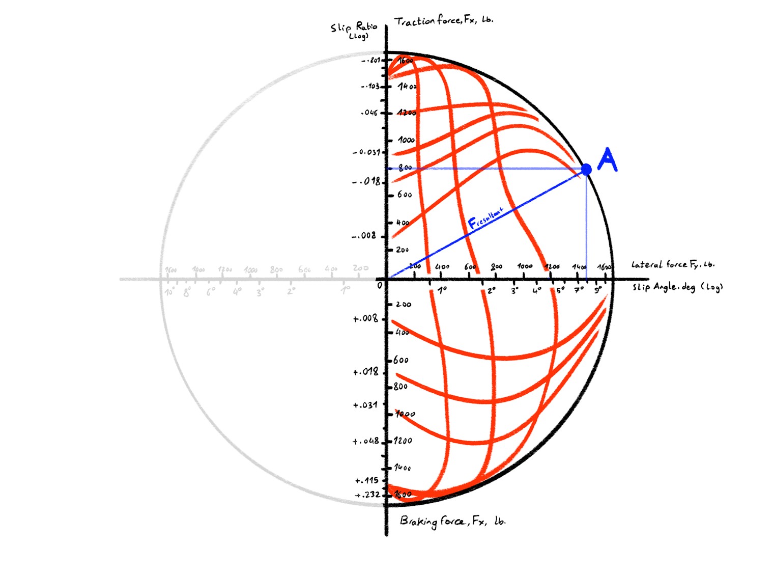
The Friction Circle
This less-than-intuitive diagram pulls the separate red curves you just saw into a single force-coordinate plot. The vertical axis is longitudinal force Fx (traction above, braking below) and is annotated with the corresponding slip-ratio values on a logarithmic scale. The horizontal axis is lateral force Fy (cornering to the right) with its matching slip-angle ticks, again on a log scale.
The circle is the classic Coulomb friction circle: in a purely Coulomb model the vector sum \( F = \sqrt{F_x^2 + F_y^2} \) would trace an isotropic limit, independent of how the tire reached that load.
The boundarie sshow the measured peak envelope for this particular tire. Inside the envelope, the red “spaghetti” are iso-slip-angle (arched) and iso-slip-ratio (concave) loci generated from empirical test data. Moving along one of these lines you see that as soon as the tire begins doing work in one direction, the available grip in the other shrinks non-uniformly: the combined-force surface is neither a neat cone nor a smooth ellipse but an irregular, load-dependent manifold.
The blue vector to point A is a snapshot operating point: the car is cornering hard (≈1,400 lb lateral) while still applying modest throttle (≈200 lb traction). The resultant sits close to the envelope; a small increase in either slip angle or slip ratio would push it outside, forcing one component of force to collapse, and for the driver to lose control.
Mathematically we can write a “budget” inequality \(F_x^2 + F_y^2 \le (\mu F_z)^2\), but the shapes here show that real tires dispense that budget in a highly nonlinear, load- and direction-sensitive way. Capturing those bulges and dips is why models like Pacejka's Magic Formula expose 10-plus coefficients per force: they are curve-fit stand-ins for thousands of points of real-world data. The challenge isn't the vector addition; it's mimicking the non-uniform dynamics hiding in the red lines so that the simulated tire lets go, regains grip, and trades forces just as the physical one does.
The good thing, however, is that you can come a long way by treating it like a simple circle and scaling things down to it.
For my implemetation, I used a two-step strategy:
Calculate longitudinal and lateral forces separately, using the respective slip ratio and slip angle as inputs to the Pacejka formula.
Normalize both forces to fit within an imaginary friction circle or ellipse. That is, if the vector sum of the forces exceeds the limit, scale them down proportionally.
Additionally, I modify the Pacejka curve parameters themselves depending on the other slip component. For example, as slip angle increases, I reduce the peak of the longitudinal curve. This adds realism by making the curves interact naturally.
This relationship is the trickiest part to get right in any tire model. And there's no universal analytical formula that solves it perfectly. Many simulation developers use proprietary models, Tire manufacturers rely on test rigs and real-world data, Academic models like Pacejka-Sharp, Derated Fiala, Dugoff are some examples of models thatprovide approximations, each with trade-offs. If you're working without a physical test bench, you have to make educated approximations.
I must also add that this is a problem I still am trying to find the best solutions for, and I would appreciate any input and suggestions about it!
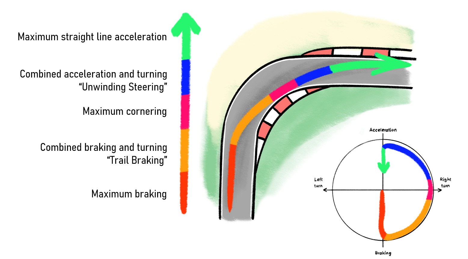
From a driver's point of view
Racing telemetry often visualizes this relationship using a G-force circle, and it maps quite well to it. The boundary of this circle (or ellipse) represents the tire's total grip. A skilled driver stays near that edge without crossing it; going beyond it means the tire breaks into full slip, and control is lost. For example:
Heavy braking → high longitudinal G, low lateral G
Mid-corner → high lateral G, almost no braking or throttle
Corner exit → throttle applied gradually as steering is unwound
This is also the logic behind trail braking, where braking is slowly reduced as turning input increases. The driver shifts their position on the traction circle smoothly, using the full potential of the tires without overloading them.
This equation reperesents the sum of all forces generated by one tire in one frame, pushed onto the chassis at the tire's contact patch position.
vertical suspension response comes from simulating a simple spring (not covered in this article, as it's not a unique problem to vehicle simulation),
longitudinal traction from throttle/brake inputs, and lateral grip from cornering.
The dynamic behavior of the tire is scaled using the slip ratio and slip angle, modulated by the coefficients \( k_0 \) and \( k_1 \), which capture how traction efficiency
changes based on vehicle state. These forces are integrated per-frame in a simulation loop to compute acceleration and update the chassis' velocity via Newton's second law.
The rest of the car, the chassis, is just a box in your rigid body physics engine.You apply the forces you calculate on it and watch it move like a car.
Now combine everything we mentioned so far, here is a demonstration from my current game engine:
Everything we've discussed so far covers the foundational systems behind vehicle simulation—engine behavior, tire dynamics, and chassis integration. But this only scratches the surface. There are many additional systems and concepts that, depending on your goals, may be worth exploring. These include suspension geometry (like camber, caster, toe), anti-roll bars and dampers, advanced tire dynamics (such as tire expansion, temperature, and wear), as well as aerodynamics, downforce and drag, dynamic aero surfaces, different differential layouts and drivetrain models, and control systems like ABS and ESP, or steering rate limitations.
There's a lot of depth to dive into as your simulation demands more detail. That said, what we've covered provides a solid holistic model of a car; one that behaves like a car and serves as a solid base to expand upon if greater fidelity is needed.
Learning about and researching this was a very fun endavor, lots of it comes from personal experience through sheer interest in motorsports and sim racing, however a large chunk comes from two great books I would definitely recommend checking out:
Race Car Vehicle Dynamics by Milliken & Milliken, and Mechanics of Pneumatic Tires by S.K. Clark
I hope this talk and article were helpful. If you have any questions, suggestions, or corrections, don't hesitate to reach out.